Trying Dgraph with genomic data

05/12/2017

In genomics we often deal with variants and samples. Variants and samples have a ‘many-to-many’ relationship and every sample will have approximately 5 million variants. So given a cohort of 1000s individuals with 10s of millions of unique variants, we are looking at approximately 5 billion sample-variant pairs! A lot of the interesting questions in genomics requires knowing about both. For example, “find all the variants for people with high blood pressure”. You can replace ‘high blood pressure’ with any clinical feature you are interested in.

Dgraph is a relatively new open source graph database that promises high performance. So lets test it out with some genomic data.

Installing Dgraph

Follow this guide

Test Data

We use Hail to generate a test dataset of 100 Samples and 1000000 Variants.

from hail import *
hc = HailContext()
vds = hc.balding_nichols_model(3, 100, 1000000)
vds = vds.variant_qc()
vds.export_genotypes('gdb_1m.tsv', 'SAMPLE=s, VARIANT=v, AF=va.qc.AF')

This creates a .csv that looks like:

SAMPLE	VARIANT	AF
0	1:1:A:C	7.50000e-01
1	1:1:A:C	7.50000e-01
0	1:3:A:C	1.00000e+00
...

ls -lah
-rw-r--r--  1 shane  staff   1.8G  5 Dec 10:31 gdb_1m.tsv

Line count:

wc -l gdb_1m.tsv
 67695719 gdb_1m.tsv

So this dataset contains about 68 million sample-variant pairs.

Loading the data

We’ll be using Dgraphs bulk loader as it dramatically improves the speed of loading large datasets. But first we’ll need to convert the CSV into an RDF which is the file format Dgraph requires as input.

I wrote a simple Go program to do this for this particular dataset (at the moment the path to the input data is hardcoded to data/gdb_1m.tsv relative to where you run the binary):

go get -u -v github.com/shusson/varsam
$GOPATH/bin/varsam

We’ll need to create a test.schema for Dgraph:

name: string @index(hash, term) .
chrom: string @index(exact) .
start: int @index(int) .
AF: float @index(float) .
variant: uid @count .

Start zero (the coordinator for the database):

dgraph zero --port_offset -2000

Load the data using the bulk loader (this took about 2 hours on my machine):

dgraph bulk -r=test.rdf -s=test.schema --map_shards=2 --reduce_shards=1 -z localhost:5080

Start server:

cd out/0
dgraph server --zero=localhost:5080 --memory_mb=2024

Simple Queries

Dgraph provides a web app on localhost:8080 which you can use to send queries. The queries are written in GraphQL+- which is a custom query language based on GraphQL.

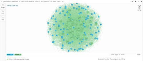
The following screenshots were captured from the Dgraph web app.

Find all variants in chromosome 1 between start position 0 and 100 for the first 3 samples

{
  sample(func: ge(count(variant), 1)) @filter(eq(sampleId, 0) OR eq(sampleId, 1) OR eq(sampleId, 3)) {
  	name
    variant @filter( eq (chrom, 1) AND ge(start, 0) AND le(start, 100)) {
    	expand(_all_) {}
  	}
  }
}

Find all variants with an Allele Frequency of 1 in the first 10 samples

{
  sample(func: ge(count(variant), 1)) @filter(ge(sampleId, 0) AND le(sampleId, 10)) {
  	name
    variant @filter( eq(AF, 1)) {
    	expand(_all_) {}
  	}
  }
}

Show the relationships of variant 1-77-A-C to all samples

{
  sample(func: ge(count(variant), 1)) {
  	name
		variant @filter( eq(name, "1-77-A-C")) {
    	expand(_all_) {}
  	}
  }
}

Conclusion

I enjoyed visualizing the data as a graph. It made me think about what other kinds of relationships we could add and how it might change the way we model genomic data. Could we show disease relationships between variants? or show the ancestral relationships between each sample? Would natural clusters emerge and would they mean anything useful?

All in all I think there is more work to do here both in terms of investigating performance and discovering new ways to visualize genomic data.